On Evaluating Neural Network Robustness
by Sarthak Gupta, Abhay Kumar, Aryan Gupta
Robustness is a critical property of deep neural networks (DNNs) that ensures correct predictions even in adversarial perturbations. Adversarial attacks exploit vulnerabilities in DNNs, where imperceptible modifications to input data can cause the model to produce incorrect outputs or misclassify inputs. Achieving robustness is essential for deploying DNNs in safety-critical applications such as autonomous driving, medical diagnosis, and cybersecurity.
Adversarial attacks pose a significant challenge in the field of deep learning. Adversaries actively seek to exploit vulnerabilities by carefully crafting perturbations that are imperceptible to humans but significantly impact the model's predictions. These attacks aim to undermine the trustworthiness and reliability of DNNs, potentially leading to severe consequences in real-world scenarios. Various adversarial attack techniques have been developed to fool neural networks. These are primarily classified into Fixed Epsilon attacks like Projected Gradient Descent (PGD) (Madry et al, 2017) and minimum norm attacks like the Fast Minimum Norm attack (FMN) (Pintor et al, 2021). Fixed ε attacks constrain the adversary to a specified magnitude of perturbation (Δ) and aim to find the optimal perturbation within this constraint. The objective is to cause misclassification or induce incorrect predictions while staying within the predefined perturbation limit. Minimum norm attacks focus on finding the smallest possible perturbation that leads to misclassification, making them optimal for finding the robustness radius around a given set of samples.
In response, various defence techniques have also been proposed to address the challenges posed by robustness-based attacks. Adversarial training, one of the most effective approaches, involves augmenting the training data with adversarial examples and retraining the model. This technique improves the model's robustness by exposing it to adversarial examples during training, enabling it to learn to generalise and make correct predictions even in the presence of perturbations. Various research works have come up with producing more and more robust models.
In this situation, model developers need to evaluate their models accurately. For this, many approaches have emerged, the most popular being empirical approaches like AutoAttack (Croce et al, 2020) and calculating the average robust radius through minimum norm attacks. However, recently, a set of approaches have gained popularity that certifiably evaluate the robust radius of a given model. The most prominent is Randomised Smoothing (Cohen et al, 2019), which calculates the maximum L2 perturbation radius up to which no perturbation can change the label of the given input. There is a considerable amount of research in each of these directions to improve the efficiency and accuracy of evaluations. However, there needs to be more literature comparing and analysing various model evaluations together. One of the aims of this paper is to fill this void and compare empirical evaluation techniques like AutoAttack and Fast Minimum Norm with certified robustness evaluation methods like randomised smoothing.
Many works consider Randomised Smoothing as a technique to defend deployed models and verifiably provide a robustness radius for a certain fraction of all queries. However, we argue that this is impractical since, even after using efficient sampling techniques, Randomised Smoothing requires hundreds to thousands of samples to verify each query. Such large numbers would be prohibitively expensive for most use cases. Thus, Randomised Smoothing and its alternatives can better be used as evaluation techniques rather than defence during deployment. How such evaluations of the smooth model help understand the robustness would be another point of discussion in our study.
FGSM(Fast Gradient Sign Method) is a simple and efficient attack that operates by calculating the gradient of the loss function with respect to the input data. It then perturbs the input by taking a step in the direction of the gradient, scaled by a small value called the epsilon. The key idea behind FGSM is to leverage the sign of the gradient to determine the direction of the perturbation, allowing for a quick generation of adversarial examples. Iterative FGSM (I-FGSM) extends this method by applying FGSM iteratively with smaller step sizes, which can lead to more potent attacks. On the other hand, PGD is an iterative attack that aims to find the maximum perturbation within a specified epsilon budget while considering the model's vulnerability to small perturbations. PGD operates by iteratively taking small steps in the direction of the gradient and then projecting the perturbation back into the epsilon ball to ensure it remains within the desired bounds. By iteratively optimizing the perturbation, PGD explores a larger space of potential adversarial examples, making it more effective and robust compared to FGSM. The main difference between FGSM and PGD lies in their optimization strategies. While FGSM is a one-step attack that calculates the gradient and perturbs the input data once, PGD takes multiple steps, each time refining the perturbation to maximize the loss function. This iterative nature of PGD allows it to overcome the defence mechanisms implemented by models, making it more potent against various defences, including adversarial training and gradient masking. However, the computational cost of PGD is higher due to the iterative process, making FGSM a more lightweight alternative in specific scenarios.
AutoAttack is a comprehensive and reliable framework for evaluating the adversarial robustness of machine learning models. Autoattack combines multiple powerful attacks to provide a more comprehensive assessment of a model's vulnerability to adversarial examples. The ensemble is comprised of two parameter-free versions of PGD, AutoPGDCE and AutoPGDDLR, and two complementary attacks, FAB (Croce et al, 2019) and Square Attack (Andriushchenko et al, 2019). The attack is because it does not require any free parameters. The attack's main strength lies in its ensemble components' diversity. Each attack within the AutoAttack framework brings a unique approach to adversarial examples. For instance, AutoPGDs are white-box attacks that aim to find any adversarial example within a specified ε-ball. On the other hand, FAB focuses on minimizing the norm of the perturbation required to achieve misclassification, making it effective even in the presence of gradient masking. Despite relying on logits' gradients, FAB has demonstrated its efficacy. Square attack, in contrast, is a black-box attack that operates based on scores rather than gradients. It performs random search within the constraints of norm-bounded perturbations, surpassing other black-box attacks in terms of query efficiency and success rate. Notably, Square Attack has proven competitive with white-box attacks, showcasing its effectiveness.
RobustBench, a widely used benchmark for model robustness, uses AutoAttack for evaluation. It contains a large number of models trained with approaches to make them robust to L-infinity, L2 and common corruptions perturbations.
Recently, minimum norm empirical attacks have also gained significance in adversarial machine learning. These attacks focus on finding the smallest perturbations that can fool a machine learning model, thereby generating adversarial examples. In the context of adversarial attacks, the term "minimum norm" refers to the objective of minimizing the norm of the perturbation added to the input sample. The norm can be defined based on various distance metrics, such as the L0 norm (count of non-zero elements), the L2 norm (Euclidean distance), or the L-infinity norm (maximum absolute difference). The key benefit of minimum norm empirical attacks, particularly when compared to fixed norm attacks, is their ability to find adversarial perturbations quickly. In fixed norm attacks, the perturbation magnitude is predefined, and the attacker iteratively adjusts the perturbation until it successfully fools the model. This process often requires multiple runs with different perturbation magnitudes, increasing computational complexity.
On the other hand, minimum norm empirical attacks, such as the Fast Minimum Norm (FMN) attack, offer a more efficient approach. The FMN attack utilizes linear extrapolation to estimate the distance between the current iteration sample and the classification boundary. By leveraging this estimation, the attack can effectively determine the minimum noise required to push the benign sample across the boundary and create an adversarial example. This strategy allows the attack to converge quickly towards finding the smallest perturbation without needing multiple iterations with varying perturbation magnitudes. Before the FMN attack gained prominence, another notable attack in the minimum norm empirical category was the DeepFool attack (Moosavi-Dezfooli et al, 2015). DeepFool iteratively "linearizes" the loss function at an input point (taking the tangent to the loss function at that point), and applies the minimal perturbation necessary to switch classes if that linear approximation were correct. This "minimal necessary perturbation" for the linear case amounts to projecting your input vector onto the "decision boundary" of your locally-linearized model.
The most widely-used certifiable evaluation method is Randomized Smoothing(RS). It adds noise to the input and uses majority voting among the model predictions for multiple noised inputs to get the final label prediction. Since shifting the centre of noised input distribution does not change the ranking of label predictions, the RS models are certifiably robust to small L2-norm-bounded perturbations. For RS, the most widely-used certification approach is the Neyman-Pearson-based certification (wikipedia page for Neyman-Pearson method). It leverages the base model's probability of predicting each class under the input noise to compute the certification. This noise distribution sampling requires our classification model to be robust to Gaussian noise. Earlier works achieved this by using noisy samples during the training process. However, later works like Denoised Smoothing(Salman et al, 2020) propose attaching a denoiser model to the base classifier, thus allowing the use of Randomized Smoothing in a plug-and-play manner without requiring retraining. This approach opens up interesting possibilities, like certifying the predictions of models deployed through APIs from the client side.
Other improvements try to get more accurate robust radius results like Double Sampling Randomized Smoothing(DSRS). In the paper Double Sampling Randomized Smoothing, the authors propose to sample the base model's prediction statistics under two different distributions and leverage the joint information to compute the certification. Since we leverage more information, our certification approach is guaranteed to be tighter (if not equal) than the most widely-used Neyman-Pearson-based approach. Theoretically, under mild assumptions, DSRS has been proved to certify √Θ robust radius under L2 norm where d is the input dimension, implying that DSRS can break the curse of dimensionality of randomized smoothing. More techniques like Input Specific Sampling(ISS)(Chen et al, 2021) have also come up to address the high computational costs associated with RS methods. The key idea of ISS is to appropriately reduce the sample size for each input instead of applying the same sample size to the certifications for all inputs.
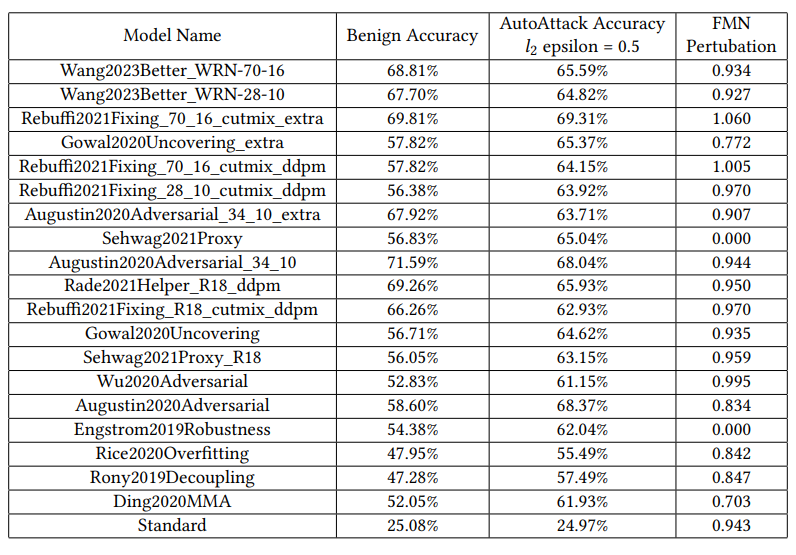
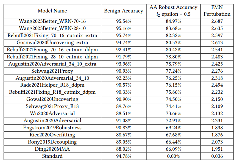
We conduct our experiments using models from the RobustBench benchmark. Specifically, we consider the models listed in the CIFAR-10 L2 perturbations section. Initially, we evaluate the RobustBench models using FMN. This evaluation is essential since it helps us differentiate between models which appear similar using the standard AutoAttack evaluation but have very different levels of robustness against adversarial samples generated with different settings. To illustrate this point, consider that two models have the same robust accuracy when evaluated with AutoAttack under L2 norm and epsilon 0.5. However, it is also possible that one has an average robust radius of 0.6 while the other has a robust radius of 0.85. Both these models would show very different behaviour when attacked by an adversary whose epsilon limit is ~0.8. In such a case, minimum norm attack-based evaluation could help differentiate between these two cases by calculating the minimum norm for each sample. An analysis of the average length of these perturbations and their standard deviation could be an excellent way to avoid such oversights. To evaluate these models using FMN, we use the standard implementation from foolbox(an open-source adversarial robustness toolbox) with 10 binary search steps and 100 total steps.
For our experiments involving randomized smoothing, we specifically use Double Sampling Randomized Smoothing(DSRS)(Li et al, 2022), which allows us to calculate a tighter radius, i.e. results which are much closer to the true robust radius(which is unknown). In the reproducibility study [Re] Double Sampling Randomized Smoothing(Gupta et al, 2023), the authors conducted a detailed DSRS method analysis. We will use many insights from this study to run the DSRS experiments. We sample 10,000 times each from two distributions since it gives an optimal trade-off between the compute requirements and verified radius. For sampling noise, we use sigma 0.5 general-gaussian distribution
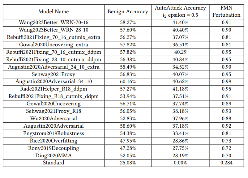
As the classifiers required for randomized smoothing must be robust to Gaussian noise, we must attach pre-trained denoisers with the classifiers from RobustBench. This is the same approach used in Denoised-Smoothing(cite) to use pre-trained classifiers for randomized smoothing. The analysis and comparison use these "denoised models" and calculate all the adversarial perturbations on the complete denoised models. Since randomized smoothing verifies the robust radius for the smoothed classifier, we cannot directly compare its verified robust radius and accuracy with that of the base classifier. Hence, we instead conduct the attacks on the smoothed classifier using AutoAttack(cite) and FMN(cite) and compare the results with the certified accuracy and radius obtained from randomized smoothing. Additionally, we compare these values with the results from the smooth classifier with results obtained from attacking the denoised base classifier. This comparison will help us understand whether the additional compute used to infer from the smooth classifier leads to better robustness.
We describe our approach to generating adversarial examples against the smooth model. Let F: Rd → Rd be the base classifier. The smooth classifier G: Rd → Rd which returns counts for each class, could be calculated as:

Generating fixed norm adversarial samples, where lcls is the classification loss, and ε is the maximum perturbation size is equivalent to:

But Algorithm 2 would mean generating adversarial samples for each x + δ, which would be very computationally expensive. To avoid this problem, we observe the transferability of adversarial examples from the base classifier to the smoothed classifier.
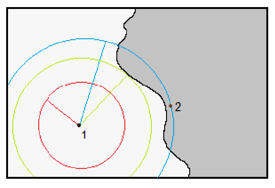
An interesting observation to make would be the difference between the minimum perturbation radius found by FMN and the robust radius calculated using DSRS. Since the L2 sphere with a robust radius resulting from DSRS must have no adversarial samples, and a successful FMN attack must produce one, the above-stated difference would be the uncertainty range for the true robust radius. The more accurate DSRS and FMN, the lesser will be the uncertainty. This is further illustrated in Figure 1.

Adversarial attacks pose a significant challenge in the field of deep learning. Adversaries actively seek to exploit vulnerabilities by carefully crafting perturbations that are imperceptible to humans but significantly impact the model's predictions. These attacks aim to undermine the trustworthiness and reliability of DNNs, potentially leading to severe consequences in real-world scenarios. Various adversarial attack techniques have been developed to fool neural networks. These are primarily classified into Fixed Epsilon attacks like Projected Gradient Descent (PGD) (Madry et al, 2017) and minimum norm attacks like the Fast Minimum Norm attack (FMN) (Pintor et al, 2021). Fixed ε attacks constrain the adversary to a specified magnitude of perturbation (Δ) and aim to find the optimal perturbation within this constraint. The objective is to cause misclassification or induce incorrect predictions while staying within the predefined perturbation limit. Minimum norm attacks focus on finding the smallest possible perturbation that leads to misclassification, making them optimal for finding the robustness radius around a given set of samples.
In response, various defence techniques have also been proposed to address the challenges posed by robustness-based attacks. Adversarial training, one of the most effective approaches, involves augmenting the training data with adversarial examples and retraining the model. This technique improves the model's robustness by exposing it to adversarial examples during training, enabling it to learn to generalise and make correct predictions even in the presence of perturbations. Various research works have come up with producing more and more robust models.
In this situation, model developers need to evaluate their models accurately. For this, many approaches have emerged, the most popular being empirical approaches like AutoAttack (Croce et al, 2020) and calculating the average robust radius through minimum norm attacks. However, recently, a set of approaches have gained popularity that certifiably evaluate the robust radius of a given model. The most prominent is Randomised Smoothing (Cohen et al, 2019), which calculates the maximum L2 perturbation radius up to which no perturbation can change the label of the given input. There is a considerable amount of research in each of these directions to improve the efficiency and accuracy of evaluations. However, there needs to be more literature comparing and analysing various model evaluations together. One of the aims of this paper is to fill this void and compare empirical evaluation techniques like AutoAttack and Fast Minimum Norm with certified robustness evaluation methods like randomised smoothing.
Many works consider Randomised Smoothing as a technique to defend deployed models and verifiably provide a robustness radius for a certain fraction of all queries. However, we argue that this is impractical since, even after using efficient sampling techniques, Randomised Smoothing requires hundreds to thousands of samples to verify each query. Such large numbers would be prohibitively expensive for most use cases. Thus, Randomised Smoothing and its alternatives can better be used as evaluation techniques rather than defence during deployment. How such evaluations of the smooth model help understand the robustness would be another point of discussion in our study.
Background
Empirical Attacks and Evaluation
Fixed norm attacks are a class of adversarial attacks that aim to deceive machine learning models by perturbing the input data within a specified norm constraint. These attacks have gained significant attention due to their ability to generate imperceptible yet impactful modifications to the input, leading to misclassification or erroneous predictions. Two prominent fixed norm attacks are FGSM (Fast Gradient Sign Method) and PGD (Projected Gradient Descent).FGSM(Fast Gradient Sign Method) is a simple and efficient attack that operates by calculating the gradient of the loss function with respect to the input data. It then perturbs the input by taking a step in the direction of the gradient, scaled by a small value called the epsilon. The key idea behind FGSM is to leverage the sign of the gradient to determine the direction of the perturbation, allowing for a quick generation of adversarial examples. Iterative FGSM (I-FGSM) extends this method by applying FGSM iteratively with smaller step sizes, which can lead to more potent attacks. On the other hand, PGD is an iterative attack that aims to find the maximum perturbation within a specified epsilon budget while considering the model's vulnerability to small perturbations. PGD operates by iteratively taking small steps in the direction of the gradient and then projecting the perturbation back into the epsilon ball to ensure it remains within the desired bounds. By iteratively optimizing the perturbation, PGD explores a larger space of potential adversarial examples, making it more effective and robust compared to FGSM. The main difference between FGSM and PGD lies in their optimization strategies. While FGSM is a one-step attack that calculates the gradient and perturbs the input data once, PGD takes multiple steps, each time refining the perturbation to maximize the loss function. This iterative nature of PGD allows it to overcome the defence mechanisms implemented by models, making it more potent against various defences, including adversarial training and gradient masking. However, the computational cost of PGD is higher due to the iterative process, making FGSM a more lightweight alternative in specific scenarios.
AutoAttack is a comprehensive and reliable framework for evaluating the adversarial robustness of machine learning models. Autoattack combines multiple powerful attacks to provide a more comprehensive assessment of a model's vulnerability to adversarial examples. The ensemble is comprised of two parameter-free versions of PGD, AutoPGDCE and AutoPGDDLR, and two complementary attacks, FAB (Croce et al, 2019) and Square Attack (Andriushchenko et al, 2019). The attack is because it does not require any free parameters. The attack's main strength lies in its ensemble components' diversity. Each attack within the AutoAttack framework brings a unique approach to adversarial examples. For instance, AutoPGDs are white-box attacks that aim to find any adversarial example within a specified ε-ball. On the other hand, FAB focuses on minimizing the norm of the perturbation required to achieve misclassification, making it effective even in the presence of gradient masking. Despite relying on logits' gradients, FAB has demonstrated its efficacy. Square attack, in contrast, is a black-box attack that operates based on scores rather than gradients. It performs random search within the constraints of norm-bounded perturbations, surpassing other black-box attacks in terms of query efficiency and success rate. Notably, Square Attack has proven competitive with white-box attacks, showcasing its effectiveness.
RobustBench, a widely used benchmark for model robustness, uses AutoAttack for evaluation. It contains a large number of models trained with approaches to make them robust to L-infinity, L2 and common corruptions perturbations.
Recently, minimum norm empirical attacks have also gained significance in adversarial machine learning. These attacks focus on finding the smallest perturbations that can fool a machine learning model, thereby generating adversarial examples. In the context of adversarial attacks, the term "minimum norm" refers to the objective of minimizing the norm of the perturbation added to the input sample. The norm can be defined based on various distance metrics, such as the L0 norm (count of non-zero elements), the L2 norm (Euclidean distance), or the L-infinity norm (maximum absolute difference). The key benefit of minimum norm empirical attacks, particularly when compared to fixed norm attacks, is their ability to find adversarial perturbations quickly. In fixed norm attacks, the perturbation magnitude is predefined, and the attacker iteratively adjusts the perturbation until it successfully fools the model. This process often requires multiple runs with different perturbation magnitudes, increasing computational complexity.
On the other hand, minimum norm empirical attacks, such as the Fast Minimum Norm (FMN) attack, offer a more efficient approach. The FMN attack utilizes linear extrapolation to estimate the distance between the current iteration sample and the classification boundary. By leveraging this estimation, the attack can effectively determine the minimum noise required to push the benign sample across the boundary and create an adversarial example. This strategy allows the attack to converge quickly towards finding the smallest perturbation without needing multiple iterations with varying perturbation magnitudes. Before the FMN attack gained prominence, another notable attack in the minimum norm empirical category was the DeepFool attack (Moosavi-Dezfooli et al, 2015). DeepFool iteratively "linearizes" the loss function at an input point (taking the tangent to the loss function at that point), and applies the minimal perturbation necessary to switch classes if that linear approximation were correct. This "minimal necessary perturbation" for the linear case amounts to projecting your input vector onto the "decision boundary" of your locally-linearized model.
Certified Defences and Evaluation
Empirical methods test the robustness by using handcrafted techniques to generate adversarial samples. On the other hand, certified defence and evaluation techniques are based on mathematical proofs, ensuring that a model following a particular methodology could be robust up to a certain level of adversarial capabilities. Given an input instance and a model, the robustness certification approach computes a robust radius, so any perturbations within the radius do not change the final prediction. By nature, the certification approach is conservative- providing a lower bound of robust radius. In contrast, the maximum robust radius for the given input instance could be much larger than the one computed by the certification approach.The most widely-used certifiable evaluation method is Randomized Smoothing(RS). It adds noise to the input and uses majority voting among the model predictions for multiple noised inputs to get the final label prediction. Since shifting the centre of noised input distribution does not change the ranking of label predictions, the RS models are certifiably robust to small L2-norm-bounded perturbations. For RS, the most widely-used certification approach is the Neyman-Pearson-based certification (wikipedia page for Neyman-Pearson method). It leverages the base model's probability of predicting each class under the input noise to compute the certification. This noise distribution sampling requires our classification model to be robust to Gaussian noise. Earlier works achieved this by using noisy samples during the training process. However, later works like Denoised Smoothing(Salman et al, 2020) propose attaching a denoiser model to the base classifier, thus allowing the use of Randomized Smoothing in a plug-and-play manner without requiring retraining. This approach opens up interesting possibilities, like certifying the predictions of models deployed through APIs from the client side.
Other improvements try to get more accurate robust radius results like Double Sampling Randomized Smoothing(DSRS). In the paper Double Sampling Randomized Smoothing, the authors propose to sample the base model's prediction statistics under two different distributions and leverage the joint information to compute the certification. Since we leverage more information, our certification approach is guaranteed to be tighter (if not equal) than the most widely-used Neyman-Pearson-based approach. Theoretically, under mild assumptions, DSRS has been proved to certify √Θ robust radius under L2 norm where d is the input dimension, implying that DSRS can break the curse of dimensionality of randomized smoothing. More techniques like Input Specific Sampling(ISS)(Chen et al, 2021) have also come up to address the high computational costs associated with RS methods. The key idea of ISS is to appropriately reduce the sample size for each input instead of applying the same sample size to the certifications for all inputs.
Experiments and Setup
On a high level, our experiments aim to analyze and compare how different robustness evaluation techniques compare and identify pitfalls into which model evaluators using standard evaluation methods could fall. This could mean identifying cases where one evaluation technique leads to over or under-estimation of robustness and providing analysis for future research.We conduct our experiments using models from the RobustBench benchmark. Specifically, we consider the models listed in the CIFAR-10 L2 perturbations section. Initially, we evaluate the RobustBench models using FMN. This evaluation is essential since it helps us differentiate between models which appear similar using the standard AutoAttack evaluation but have very different levels of robustness against adversarial samples generated with different settings. To illustrate this point, consider that two models have the same robust accuracy when evaluated with AutoAttack under L2 norm and epsilon 0.5. However, it is also possible that one has an average robust radius of 0.6 while the other has a robust radius of 0.85. Both these models would show very different behaviour when attacked by an adversary whose epsilon limit is ~0.8. In such a case, minimum norm attack-based evaluation could help differentiate between these two cases by calculating the minimum norm for each sample. An analysis of the average length of these perturbations and their standard deviation could be an excellent way to avoid such oversights. To evaluate these models using FMN, we use the standard implementation from foolbox(an open-source adversarial robustness toolbox) with 10 binary search steps and 100 total steps.
For our experiments involving randomized smoothing, we specifically use Double Sampling Randomized Smoothing(DSRS)(Li et al, 2022), which allows us to calculate a tighter radius, i.e. results which are much closer to the true robust radius(which is unknown). In the reproducibility study [Re] Double Sampling Randomized Smoothing(Gupta et al, 2023), the authors conducted a detailed DSRS method analysis. We will use many insights from this study to run the DSRS experiments. We sample 10,000 times each from two distributions since it gives an optimal trade-off between the compute requirements and verified radius. For sampling noise, we use sigma 0.5 general-gaussian distribution
As the classifiers required for randomized smoothing must be robust to Gaussian noise, we must attach pre-trained denoisers with the classifiers from RobustBench. This is the same approach used in Denoised-Smoothing(cite) to use pre-trained classifiers for randomized smoothing. The analysis and comparison use these "denoised models" and calculate all the adversarial perturbations on the complete denoised models. Since randomized smoothing verifies the robust radius for the smoothed classifier, we cannot directly compare its verified robust radius and accuracy with that of the base classifier. Hence, we instead conduct the attacks on the smoothed classifier using AutoAttack(cite) and FMN(cite) and compare the results with the certified accuracy and radius obtained from randomized smoothing. Additionally, we compare these values with the results from the smooth classifier with results obtained from attacking the denoised base classifier. This comparison will help us understand whether the additional compute used to infer from the smooth classifier leads to better robustness.
We describe our approach to generating adversarial examples against the smooth model. Let F: Rd → Rd be the base classifier. The smooth classifier G: Rd → Rd which returns counts for each class, could be calculated as:

Algorithm 1

Algorithm 2
An interesting observation to make would be the difference between the minimum perturbation radius found by FMN and the robust radius calculated using DSRS. Since the L2 sphere with a robust radius resulting from DSRS must have no adversarial samples, and a successful FMN attack must produce one, the above-stated difference would be the uncertainty range for the true robust radius. The more accurate DSRS and FMN, the lesser will be the uncertainty. This is further illustrated in Figure 1.

Figure 1: An illustration describing the situation when DSRS and FMN are used to evaluate a given point in the input space. The white and gray regions belong to different classes. By attacking the original point 1, FMN finds an adversarial point 2 near the classification boundary. The red circle is the hypersphere with the certified radius devised from DSRS. It must be the case that the true robust radius(green) must lie between or be equal to the radius found by DSRS and the minimum perturbation norm found by FMN(Blue)
Results

Results Table 1: Evaluations on base classifier without denoisers

Results Table 2: Evaluations on base classifier with denoisers
